Grover's algorithm
Grover's algorithm searches an unstructured list of \( N \) items in about \( \sqrt{N} \) steps, where any classical search needs about \( N \). It's the most broadly applicable quantum algorithm there is: anything you can phrase as "recognize the right answer when you see it" - database search, constraint solving, brute-forcing a key - gets this quadratic speedup.
Why this exists
Imagine a phone book with a million entries, sorted by name, and you have only a phone number. No sorting helps you; the entries are in effectively random order with respect to what you're searching by. Classically your only move is to check entries one by one: on average half a million checks, worst case a million.
Grover's algorithm finds the entry in about \( \frac{\pi}{4}\sqrt{N} \approx 785 \) steps for a million items. Quadratic rather than exponential speedup, but with almost no fine print: it doesn't need the problem to have any special structure, just a way to recognize the answer. That recognition test becomes the oracle.
One important expectation to set: Grover's doesn't "look at all items and pick the right one" in a single step. It gradually amplifies the right answer's amplitude over many iterations while the wrong answers' amplitudes shrink. The magic is in how few iterations that takes.
What you need to know first
- Oracles - covered in Deutsch-Jozsa: what an oracle is. Grover's uses a phase oracle: instead of writing the answer into an ancilla, it flips the sign of the marked item's amplitude and leaves everything else alone. (Any ordinary recognizing circuit converts into a phase oracle with the \( |-\rangle \) ancilla trick from that same page.)
- Amplitudes vs probabilities - a state's amplitude is the signed (in general complex) number whose square gives the probability. Grover's works entirely on amplitudes, using the sign flips that probabilities can't see.
- Mean/average of a list of numbers - genuinely just that. The diffusion step reflects amplitudes about their average. Khan Academy's statistics basics covers it in the first lesson.
- Some trigonometry helps for the iteration-count analysis: unit circle and sine.
How it works, step by step
Search space: all \( N = 2^n \) bitstrings on \( n \) qubits. One of them, \( |w\rangle \) (the "winner"), is marked by the oracle.
- Superpose everything: H on every qubit. All \( N \) items now have equal amplitude \( \frac{1}{\sqrt{N}} \).
- Grover iteration (repeat \( \approx \frac{\pi}{4}\sqrt{N} \) times):
- Oracle: flip the sign of the winner's amplitude. Nothing measurable changes yet - probabilities are amplitude squared - but the winner is now tagged.
- Diffusion (inversion about the mean): replace every amplitude \( a \) with \( 2\bar{a} - a \), where \( \bar{a} \) is the average of all amplitudes. Everything reflects through the average. The winner, sitting far below the average after its sign flip, gets catapulted far above it; everyone else shrinks slightly.
- Measure: the winner comes out with high probability.
Why can't you just iterate forever until the winner has probability 1? Because the process is a rotation, not a ratchet - overshoot the right count and the winner's amplitude starts decreasing again. The analysis below makes this precise.
The math
The whole evolution lives in a 2D plane spanned by \( |w\rangle \) (the winner) and the uniform superposition of all the losers. Define \( \sin\theta = \frac{1}{\sqrt{N}} \); the starting state sits at angle \( \theta \) above the all-losers axis. Each Grover iteration is two reflections (oracle = reflect across the losers axis, diffusion = reflect across the starting state), and two reflections make a rotation by \( 2\theta \) toward the winner.
After \( k \) iterations the probability of measuring the winner is
You want \( (2k+1)\theta \approx \frac{\pi}{2} \), giving the optimal iteration count
That square root is the entire speedup, and the sine curve explains the overshoot warning: keep iterating past the peak and \( P(w) \) falls back down. Grover's is provably optimal, too - no quantum algorithm can do unstructured search in fewer than \( \Omega(\sqrt{N}) \) queries, so the quadratic speedup is the final word.
A worked example
Take \( n = 2 \), so \( N = 4 \) items, with winner \( |11\rangle \). Here \( \sin\theta = \frac{1}{2} \) means \( \theta = 30° \), and \( (2k+1)\theta = 90° \) at exactly \( k = 1 \): one iteration finds the winner with certainty. Track the four amplitudes by hand:
| \( \lvert 00\rangle \) | \( \lvert 01\rangle \) | \( \lvert 10\rangle \) | \( \lvert 11\rangle \) | |
|---|---|---|---|---|
| After H layer | 0.5 | 0.5 | 0.5 | 0.5 |
| After oracle | 0.5 | 0.5 | 0.5 | −0.5 |
| After diffusion | 0 | 0 | 0 | 1.0 |
The diffusion arithmetic: the average of \( (0.5, 0.5, 0.5, -0.5) \) is \( \bar{a} = 0.25 \). Each amplitude becomes \( 2\bar{a} - a \): the losers get \( 0.5 - 0.5 = 0 \), the winner gets \( 0.5 + 0.5 = 1.0 \). Every shot now returns 11.
The circuit
For the \( N = 4 \), winner-\( |11\rangle \) example, build on 2 qubits (or load it from the Ready algorithms panel). A controlled-Z (CZ) is a Z gate with a control attached; it flips the sign of \( |11\rangle \) only, which is exactly the oracle we need.
- Superpose: H on
q[0]andq[1] - Oracle: CZ between
q[0]andq[1] - Diffusion: H on both, X on both, CZ, X on both, H on both
- Measure both qubits -
11every time
To mark a different winner, sandwich the oracle's CZ with X gates on the qubits that should read 0 (e.g. winner \( |01\rangle \): X on q[1], CZ, X on q[1]).
References for the circuit layout: Wikipedia: Grover's algorithm and IBM Quantum Learning: Grover's algorithm.
The circuit in code
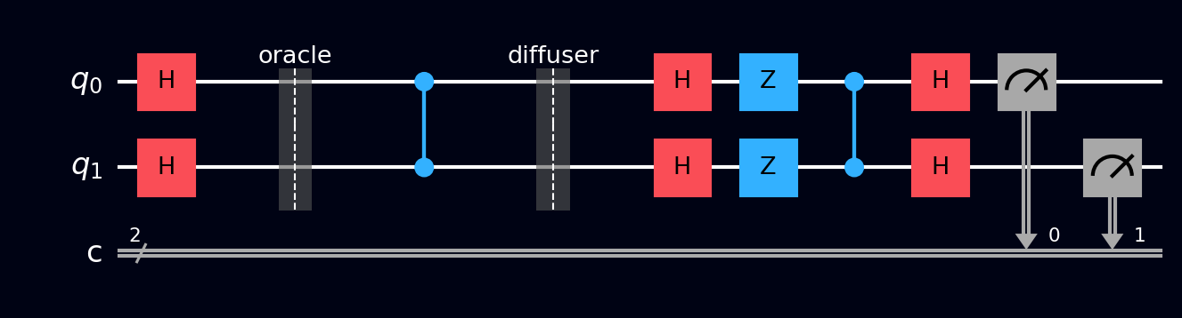
The \( N = 4 \), winner-\( |11\rangle \) circuit (one Grover iteration, 2 qubits). Barriers separate the three phases: superposition, oracle, and diffusion + measurement.
OPENQASM 2.0;
include "qelib1.inc";

qreg q[2];
creg c[2];

// Superpose
h q[0];
h q[1];
barrier q;

// Oracle: flip the sign of |11>
cz q[0], q[1];
barrier q;

// Diffusion: inversion about the mean
h q[0];
h q[1];
x q[0];
x q[1];
cz q[0], q[1];
x q[0];
x q[1];
h q[0];
h q[1];

measure q -> c;
OPENQASM 3.0;
include "stdgates.inc";

qubit[2] q;
bit[2] c;

// Superpose
h q[0];
h q[1];
barrier q;

// Oracle: flip the sign of |11>
cz q[0], q[1];
barrier q;

// Diffusion: inversion about the mean
h q[0];
h q[1];
x q[0];
x q[1];
cz q[0], q[1];
x q[0];
x q[1];
h q[0];
h q[1];

c = measure q;
from qiskit import QuantumCircuit
from qiskit_aer import AerSimulator

qc = QuantumCircuit(2, 2)

# Uniform superposition over all four items
qc.h([0, 1])
qc.barrier()

# Oracle: CZ flips the sign of |11> only.
# Replace with your own recognition test as a phase flip.
qc.cz(0, 1)
qc.barrier()

# Diffusion (reflect about the uniform state):
# H-X maps the uniform state onto |11>, CZ flips everything
# except that reference, then X-H maps back.
qc.h([0, 1])
qc.x([0, 1])
qc.cz(0, 1)
qc.x([0, 1])
qc.h([0, 1])

qc.measure([0, 1], [0, 1])

# N=4 hits certainty at k=1 iteration. Output: {'11': 1024}
counts = AerSimulator().run(qc, shots=1024).result().get_counts()
print(counts)
import cirq

q = cirq.LineQubit.range(2)

circuit = cirq.Circuit()
# Superpose
circuit.append([cirq.H(q[0]), cirq.H(q[1])])
circuit.append(cirq.ops.Moment())  # barrier

# Oracle: flip the sign of |11>
circuit.append(cirq.CZ(q[0], q[1]))
circuit.append(cirq.ops.Moment())  # barrier

# Diffusion: inversion about the mean
circuit.append([cirq.H(q[0]), cirq.H(q[1])])
circuit.append([cirq.X(q[0]), cirq.X(q[1])])
circuit.append(cirq.CZ(q[0], q[1]))
circuit.append([cirq.X(q[0]), cirq.X(q[1])])
circuit.append([cirq.H(q[0]), cirq.H(q[1])])

circuit.append(cirq.measure(*q, key='result'))
print(circuit)
namespace QompileCircuit {
    open Microsoft.Quantum.Canon;
    open Microsoft.Quantum.Intrinsic;

    operation Circuit() : Result[] {
        use q = Qubit[2];
        mutable c = [Zero, size = 2];

        // Superpose
        H(q[0]);
        H(q[1]);

        // Oracle: flip the sign of |11>
        CZ(q[0], q[1]);

        // Diffusion: inversion about the mean
        H(q[0]);
        H(q[1]);
        X(q[0]);
        X(q[1]);
        CZ(q[0], q[1]);
        X(q[0]);
        X(q[1]);
        H(q[0]);
        H(q[1]);

        set c w/= 0 <- M(q[0]);
        set c w/= 1 <- M(q[1]);

        ResetAll(q);
        return c;
    }
}
What you'll see
- Probabilities - a single bar at 100% on
11. For a genuinely instructive view, place snapshots between stages and watch the histogram morph from flat, to flat (the oracle's sign flip is invisible here), to fully concentrated. - Q-Sphere - after the oracle: four equal points, with \( |11\rangle \) phase-colored opposite to the rest. This is the clearest picture of "tagged but not yet amplified."
- Statevector - the table from the worked example, live: \( (0.5, 0.5, 0.5, 0.5) \) → \( (0.5, 0.5, 0.5, -0.5) \) → \( (0, 0, 0, 1) \).