Simon's algorithm
Simon's algorithm finds a hidden XOR-mask exponentially faster than any classical method - not "somewhat faster" like Deutsch-Jozsa or Bernstein-Vazirani, but the difference between a handful of queries and more queries than the universe has time for. Historically, this was the result that inspired Shor to build his factoring algorithm: both are, at heart, period-finding algorithms.
Why this exists
The game: a mystery function \( f \) maps \( n \)-bit strings to \( n \)-bit strings, with a promise: there's a secret nonzero string \( s \) such that
So \( f \) is two-to-one: the inputs pair up (each \( x \) with its partner \( x \oplus s \)), and each pair shares one output value. You could call \( s \) a period, but with respect to XOR instead of ordinary addition: shifting the input by \( s \) (in the XOR sense) leaves the output unchanged. Your job is to find \( s \).
Classically this is brutally hard. The only way to learn anything is to find a collision - two inputs with the same output - and until you stumble on one, the outputs look like random noise. By the birthday-paradox argument you need around \( \sqrt{2^n} = 2^{n/2} \) queries. For \( n = 128 \), that's \( 2^{64} \) function calls.
Simon's algorithm needs about \( n \) queries. For \( n = 128 \): roughly 128 calls plus a bit of high-school-style algebra. That's an exponential separation, proven, and it was the first of its kind.
What you need to know first
- Oracles and how quantum circuits package functions - covered in Deutsch-Jozsa: what an oracle is. One difference here: the output register is \( n \) bits wide, not a single ancilla, and there's no \( |-\rangle \) trick - Simon's uses the output register in the plain "write the answer" way.
- XOR as bitwise addition mod 2 - Khan Academy's XOR primer.
- The Hadamard identity \( H^{\otimes n}|x\rangle = \frac{1}{\sqrt{2^n}}\sum_y (-1)^{x \cdot y}|y\rangle \) - introduced on the Bernstein-Vazirani page.
- Solving small systems of linear equations - the classical post-processing step. Same idea as ordinary systems of equations, except every number is 0 or 1 and addition is XOR.
How it works, step by step
Two registers of \( n \) qubits each: input and output. Each run of the circuit:
- Superpose the inputs: H on every input qubit.
- One oracle call: compute \( f \) into the output register: \( \sum_x |x\rangle|f(x)\rangle \). The two registers are now entangled.
-
Forget the output: measure (or simply ignore) the output register. Whatever value \( f(x_0) \) it shows, the input register collapses to the two partners that share it:
\[ \frac{|x_0\rangle + |x_0 \oplus s\rangle}{\sqrt{2}} \]The secret is now inside the input register - as the difference between two superposed strings - but measuring right away would just give a random one of the two and teach you nothing.
-
Interfere: H on every input qubit.
-
Measure the input register. The result is a random string \( y \) satisfying
\[ y \cdot s = 0 \pmod 2 \]One run gives one equation constraining \( s \). It doesn't reveal \( s \), but it cuts the possibilities in half.
-
Repeat and solve (classical part): run the circuit until you've collected \( n - 1 \) independent equations, then solve the linear system mod 2 for \( s \). On average this takes only a little over \( n \) runs.
The math
Why does step 5 only ever produce \( y \) with \( y \cdot s = 0 \)? Apply the Hadamard identity to the collapsed state from step 3. The amplitude landing on \( |y\rangle \) is proportional to
- If \( s \cdot y = 1 \): the bracket is \( 1 - 1 = 0 \). That outcome is impossible - the two paths cancel exactly.
- If \( s \cdot y = 0 \): the bracket is \( 2 \). Those outcomes survive, all equally likely.
Interference doesn't hand you \( s \) directly; it hands you a perfectly clean constraint on \( s \), every single run. The randomness (which \( y \) you get) is harmless; the guarantee (\( y \cdot s = 0 \)) is what you keep.
A worked example
Take \( n = 2 \), secret \( s = 11 \), and \( f(x_1 x_0) = x_1 \oplus x_0 \) written into a single output bit (for \( n = 2 \) a 1-bit output is enough). Check the promise: \( f(00) = f(11) = 0 \) and \( f(01) = f(10) = 1 \) - inputs pair up exactly by \( \oplus 11 \). The oracle is two CNOTs: q[0] → q[2] and q[1] → q[2].
Run the circuit. Suppose the output register measures 0: the input register collapses to \( \frac{|00\rangle + |11\rangle}{\sqrt{2}} \). After the final Hadamards (do the algebra or trust the boxed formula), only \( |00\rangle \) and \( |11\rangle \) remain possible - both satisfy \( y \cdot 11 = 0 \), since \( y_1 \oplus y_0 = 0 \) for both.
Now the classical step. The outcome \( y = 00 \) is the trivial equation "0 = 0" and teaches nothing; keep sampling until you get \( y = 11 \), which says \( s_1 \oplus s_0 = 0 \), i.e. the secret's two bits are equal. Combined with the promise \( s \neq 00 \), the only option left is \( s = 11 \). Found it.
The circuit
For the \( n = 2 \), \( s = 11 \) example, build on 3 qubits (q[0], q[1] input; q[2] output), or load it from the Ready algorithms panel:
- H on
q[0]andq[1] - Oracle: CNOT
q[0]→q[2], CNOTq[1]→q[2] - Measure
q[2](optional - discarding it works too) - H on
q[0]andq[1] - Measure
q[0]andq[1]- you'll only ever see00or11, each about half the time;01and10never appear
References for the circuit layout: Wikipedia: Simon's problem and IBM Quantum Learning: Quantum query algorithms.
The circuit in code
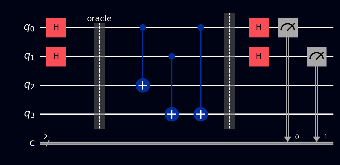
The \( n = 2 \), \( s = 11 \) circuit (4 qubits: 2 input + 2 output). Barriers separate the three phases: superpose inputs, oracle, and interference + measurement.
OPENQASM 2.0;
include "qelib1.inc";

qreg q[3];
creg c[2];

// Superpose the input register
h q[0];
h q[1];
barrier q;

// Oracle: f(x) = x0 XOR x1 (two-to-one with mask s = 11)
cx q[0], q[2];
cx q[1], q[2];
barrier q;

// Interfere and measure input register only
h q[0];
h q[1];
measure q[0] -> c[0];
measure q[1] -> c[1];
OPENQASM 3.0;
include "stdgates.inc";

qubit[3] q;
bit[2] c;

// Superpose the input register
h q[0];
h q[1];
barrier q;

// Oracle: f(x) = x0 XOR x1
cx q[0], q[2];
cx q[1], q[2];
barrier q;

// Interfere and measure input register only
h q[0];
h q[1];
c[0] = measure q[0];
c[1] = measure q[1];
from qiskit import QuantumCircuit
from qiskit_aer import AerSimulator

n = 2                      # input size; secret s = 11
qc = QuantumCircuit(n + 1, n)

# All inputs in superposition — one oracle call covers all 2^n inputs
qc.h(range(n))
qc.barrier()

# Oracle: f(x) = x0 XOR x1 (two-to-one with mask s = 11).
# No |-> ancilla trick — the answer is genuinely written into q[2],
# and it's the resulting entanglement that does the work.
qc.cx(0, n)
qc.cx(1, n)
qc.barrier()

# Output register isn't measured — discarding an entangled register
# has the same collapsing effect as measuring it
qc.h(range(n))
qc.measure(range(n), range(n))

# Only 00 and 11 appear (~50/50); 01 and 10 are killed by interference.
# Collect n-1 independent nonzero results, solve mod-2 to recover s.
counts = AerSimulator().run(qc, shots=1024).result().get_counts()
print(counts)
import cirq

q = cirq.LineQubit.range(3)

circuit = cirq.Circuit()
# Superpose the input register
circuit.append(cirq.H(q[0]))
circuit.append(cirq.H(q[1]))
circuit.append(cirq.ops.Moment())  # barrier

# Oracle: f(x) = x0 XOR x1
circuit.append(cirq.CNOT(q[0], q[2]))
circuit.append(cirq.CNOT(q[1], q[2]))
circuit.append(cirq.ops.Moment())  # barrier

# Interfere and measure input register only
circuit.append(cirq.H(q[0]))
circuit.append(cirq.H(q[1]))
circuit.append(cirq.measure(q[0], q[1], key='result'))
print(circuit)
namespace QompileCircuit {
    open Microsoft.Quantum.Canon;
    open Microsoft.Quantum.Intrinsic;

    operation Circuit() : Result[] {
        use q = Qubit[3];
        mutable c = [Zero, size = 2];

        // Superpose the input register
        H(q[0]);
        H(q[1]);

        // Oracle: f(x) = x0 XOR x1
        CNOT(q[0], q[2]);
        CNOT(q[1], q[2]);

        // Interfere and measure input register only
        H(q[0]);
        H(q[1]);
        set c w/= 0 <- M(q[0]);
        set c w/= 1 <- M(q[1]);

        ResetAll(q);
        return c;
    }
}
What you'll see
- Probabilities - only the outcomes with \( y \cdot s = 0 \) appear, all equal; the forbidden half of the histogram is exactly empty.
- Q-Sphere - after the oracle, the entangled input-output state shows four branches; after the final Hadamards, only the allowed \( y \) values remain.
- Statevector - the cancellations are visible directly: amplitudes on \( y \cdot s = 1 \) outcomes are exactly zero, not just small.