Quantum teleportation
Quantum teleportation transmits the exact quantum state of a qubit from one place to another without physically sending the qubit itself. It consumes one pre-shared entangled pair and two classical bits, and despite the name, nothing travels faster than light - the protocol can't complete until the classical bits arrive by ordinary means.
Why this exists
Suppose Alice holds a qubit in some state \( |\psi\rangle = \alpha|0\rangle + \beta|1\rangle \) and wants Bob to have it. Two obvious ideas fail:
- "Just measure it and tell Bob the result." Measuring collapses the state to a plain 0 or 1. The amplitudes \( \alpha \) and \( \beta \) - the actual information - are destroyed, and one measurement of one copy can never reveal them.
- "Just copy it and send the copy." Impossible. The no-cloning theorem says no quantum operation can duplicate an arbitrary unknown state. (The one-line reason: quantum operations are linear, and a machine that maps \( |\psi\rangle \mapsto |\psi\rangle|\psi\rangle \) for every \( |\psi\rangle \) would have to be quadratic in the amplitudes. No such linear machine exists.)
Teleportation is the workaround. It moves the state without measuring it directly and without copying it - the original is necessarily destroyed in the process, which is exactly what no-cloning demands. This isn't just a party trick: teleportation is the basic subroutine behind quantum repeaters, networked quantum computers, and many error-correction schemes.
What you need to know first
- Bell states - the protocol runs on a shared \( |\Phi^+\rangle \) pair; see Bell states.
- What \( \alpha \) and \( \beta \) are - a general qubit state is \( \alpha|0\rangle + \beta|1\rangle \) where \( \alpha, \beta \) are complex numbers with \( |\alpha|^2 + |\beta|^2 = 1 \). \( |\alpha|^2 \) is the probability of measuring 0, \( |\beta|^2 \) of measuring 1. If complex numbers are rusty, Khan Academy's complex numbers unit covers everything needed here.
- Classically controlled gates - the last step applies gates conditioned on measurement results. Qompile supports this directly; see Controls and conditionals and the Conditional (if) page.
How it works, step by step
Three qubits: q[0] is Alice's message qubit in the unknown state \( |\psi\rangle \), and q[1] (Alice's) + q[2] (Bob's) form a shared Bell pair.
- Share entanglement: create \( |\Phi^+\rangle \) between
q[1]andq[2](H onq[1], CNOTq[1]→q[2]). Bob takesq[2]far away. - Bell measurement: Alice entangles her message qubit with her half of the pair - CNOT
q[0]→q[1], then H onq[0]- and measures both of her qubits. She gets two ordinary classical bits \( (m_0, m_1) \), each 0 or 1 with equal probability. - Send two classical bits: Alice sends \( m_0, m_1 \) to Bob over any classical channel (phone, internet, carrier pigeon).
- Correction: Bob applies X to his qubit if \( m_1 = 1 \), then Z if \( m_0 = 1 \). His qubit is now in exactly the state \( |\psi\rangle \). Alice's original, meanwhile, was destroyed by her measurement - the state moved, it wasn't copied.
Two things worth stressing:
- No faster-than-light communication. Until the classical bits arrive, Bob's qubit looks completely random to him. The entanglement alone carries no usable message.
- The state is never learned. Nobody ever finds out what \( \alpha \) and \( \beta \) were. The protocol moves the state blindly, which is the only way no-cloning allows.
The math
Write the full three-qubit state before Alice's measurement. Starting point:
Apply CNOT q[0] → q[1], then H on q[0], expand, and group the terms by what Alice's two qubits look like. The algebra (worth doing once by hand) lands on:
Read this line carefully - it's the whole protocol in one equation. Whatever pair of bits Alice measures, Bob's qubit (the right-hand factor) is almost \( |\psi\rangle \), off by at most a bit flip and/or a sign flip:
| Alice measures \( (m_0, m_1) \) | Bob holds | Bob's fix |
|---|---|---|
| 00 | \( \alpha\lvert 0\rangle + \beta\lvert 1\rangle \) | nothing |
| 01 | \( \alpha\lvert 1\rangle + \beta\lvert 0\rangle \) | X |
| 10 | \( \alpha\lvert 0\rangle - \beta\lvert 1\rangle \) | Z |
| 11 | \( \alpha\lvert 1\rangle - \beta\lvert 0\rangle \) | X then Z |
Each outcome happens with probability \( \frac{1}{4} \) regardless of \( \alpha, \beta \) - which is why the measurement results leak nothing about the state.
A worked example
Give the message qubit a concrete, recognizable state: apply RY(\( \pi/3 \)) to q[0], producing
so \( |\psi\rangle \) measures 0 with probability 75% and 1 with probability 25%. Run the full protocol, then measure Bob's qubit q[2] over many shots: it shows the same 75/25 split, no matter which of the four outcomes Alice's measurement produced along the way. The 75/25 fingerprint has moved from q[0] to q[2].
The circuit
Build on 3 qubits (or load it from the Ready algorithms panel):
- Prepare the message: RY(\( \pi/3 \)) on
q[0](any state works; this one is easy to recognize) - Share the pair: H on
q[1], CNOTq[1]→q[2] - Bell measurement: CNOT
q[0]→q[1], H onq[0], measureq[0]→c0andq[1]→c1 - Corrections: X on
q[2]conditioned onc1 = 1, then Z onq[2]conditioned onc0 = 1 - Verify: measure
q[2]
References for the circuit layout: Wikipedia: Quantum teleportation and IBM Quantum Learning: Entanglement in action.
The circuit in code
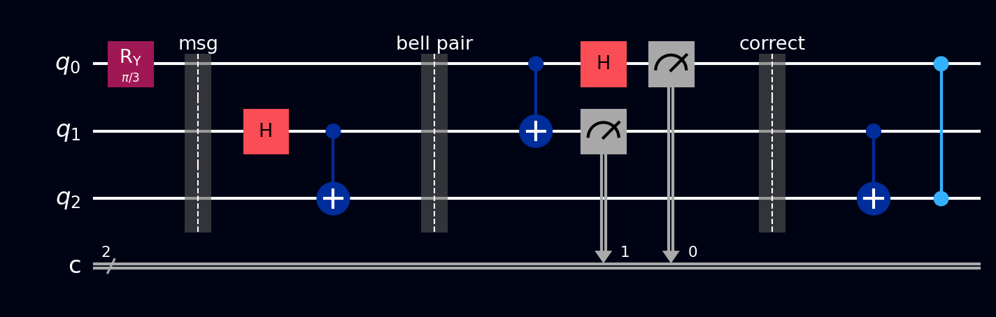
Barriers separate the four phases: prepare the message, share the Bell pair, Bell measurement + corrections, and verification.
OPENQASM 2.0;
include "qelib1.inc";

qreg q[3];
creg c[3];

// Prepare the message state on q0
ry(pi/3) q[0];
barrier q;

// Share the Bell pair between q1 (Alice) and q2 (Bob)
h q[1];
cx q[1], q[2];
barrier q;

// Alice's Bell measurement
cx q[0], q[1];
h q[0];
measure q[0] -> c[0];
measure q[1] -> c[1];

// Bob's corrections
if(c[1]==1) x q[2];
if(c[0]==1) z q[2];

// Verify
measure q[2] -> c[2];
OPENQASM 3.0;
include "stdgates.inc";

qubit[3] q;
bit[3] c;

// Prepare the message state on q0
ry(pi/3) q[0];
barrier q;

// Share the Bell pair between q1 (Alice) and q2 (Bob)
h q[1];
cx q[1], q[2];
barrier q;

// Alice's Bell measurement
cx q[0], q[1];
h q[0];
c[0] = measure q[0];
c[1] = measure q[1];

// Bob's corrections
if (c[1] == 1) x q[2];
if (c[0] == 1) z q[2];

// Verify
c[2] = measure q[2];
from math import pi
from qiskit import QuantumCircuit
from qiskit_aer import AerSimulator

qc = QuantumCircuit(3, 3)

# Prepare a recognizable 75/25 message state on q0
qc.ry(pi / 3, 0)
qc.barrier()

# Shared Bell pair: q1 stays with Alice, q2 goes to Bob
qc.h(1)
qc.cx(1, 2)
qc.barrier()

# Alice entangles her message qubit with her half, then measures
qc.cx(0, 1)
qc.h(0)
qc.measure(0, 0)
qc.measure(1, 1)

# Bob's classically controlled corrections — real feed-forward:
# the gate only fires when the matching classical bit came out 1
with qc.if_test((qc.clbits[1], 1)):
    qc.x(2)
with qc.if_test((qc.clbits[0], 1)):
    qc.z(2)

# Verify: Bob's qubit should show the same 75/25 fingerprint
qc.measure(2, 2)

# Qiskit prints bits as c2 c1 c0 — summing over Alice's bits,
# Bob's bit (leftmost char) is 0 ~75% and 1 ~25%
counts = AerSimulator().run(qc, shots=4096).result().get_counts()
print(counts)
import cirq
import numpy as np

q = cirq.LineQubit.range(3)

circuit = cirq.Circuit()
# Prepare the message state on q0
circuit.append(cirq.ry(np.pi / 3).on(q[0]))
circuit.append(cirq.ops.Moment())  # barrier

# Share the Bell pair between q1 (Alice) and q2 (Bob)
circuit.append(cirq.H(q[1]))
circuit.append(cirq.CNOT(q[1], q[2]))
circuit.append(cirq.ops.Moment())  # barrier

# Alice's Bell measurement
circuit.append(cirq.CNOT(q[0], q[1]))
circuit.append(cirq.H(q[0]))
circuit.append(cirq.measure(q[0], key='m0'))
circuit.append(cirq.measure(q[1], key='m1'))

# Bob's corrections (classically controlled)
circuit.append(cirq.X(q[2]).with_classical_controls('m1'))
circuit.append(cirq.Z(q[2]).with_classical_controls('m0'))

# Verify
circuit.append(cirq.measure(q[2], key='result'))
print(circuit)
namespace QompileCircuit {
    open Microsoft.Quantum.Canon;
    open Microsoft.Quantum.Intrinsic;
    open Microsoft.Quantum.Math;

    operation Circuit() : Result[] {
        use q = Qubit[3];
        mutable c = [Zero, size = 3];

        // Prepare the message state on q0
        Ry(PI() / 3.0, q[0]);

        // Share the Bell pair between q1 (Alice) and q2 (Bob)
        H(q[1]);
        CNOT(q[1], q[2]);

        // Alice's Bell measurement
        CNOT(q[0], q[1]);
        H(q[0]);
        set c w/= 0 <- M(q[0]);
        set c w/= 1 <- M(q[1]);

        // Bob's corrections
        if (c[1] == One) { X(q[2]); }
        if (c[0] == One) { Z(q[2]); }

        // Verify
        set c w/= 2 <- M(q[2]);

        ResetAll(q);
        return c;
    }
}
What you'll see
- Probabilities - all eight outcomes appear, but grouped by Bob's bit they reproduce the message's 75/25 split, evenly spread across Alice's four equally likely outcomes.
- Phase disks - drop a snapshot after step 2 and
q[0]shows the lopsided message state whileq[1]/q[2]sit at 50/50; after the corrections, the lopsided disk has moved toq[2]. - Statevector - before Alice measures, eight amplitudes; the grouped structure of the boxed equation above is directly visible in which amplitudes share values.