VQE¶
The Variational Quantum Eigensolver estimates the lowest energy state of a molecule or quantum system - its ground state - by teaming a short, tunable quantum circuit with an ordinary classical optimizer. It's the flagship quantum chemistry algorithm for today's noisy hardware, and the sister algorithm of QAOA: same hybrid quantum-classical loop, aimed at physics instead of optimization.
Why this exists¶
An enormous amount of chemistry and materials science boils down to one number: the ground-state energy. It decides which molecules are stable, how fast reactions run, how strongly a drug candidate binds to its target, whether a material superconducts. And computing it classically gets exponentially harder as molecules grow, because the number of quantum configurations to track doubles with every orbital - this is precisely the problem that made Feynman propose quantum computers in the first place: simulate quantum systems with a quantum system.
QPE can extract these energies with textbook precision, but it demands long circuits and error-corrected hardware that doesn't exist yet. VQE (introduced in 2014) makes the opposite trade: many short circuit runs, with a classical optimizer doing the heavy lifting between them. Short circuits survive noise, which is why VQE became the standard near-term approach.
What you need to know first¶
Hamiltonians¶
A Hamiltonian \( H \) is the operator that represents a system's total energy - think of it as the quantum score sheet, as on the QAOA page. Its eigenvalues are the energies the system is allowed to have, its eigenvectors are the corresponding states, and the smallest eigenvalue \( E_0 \) with its eigenvector is the ground state. On a quantum computer, any Hamiltonian is written as a weighted sum of Pauli strings - products of X, Y, Z, and identity gates, like \( 0.5\, Z \otimes Z \) or \( 0.3\, X \otimes I \).
Eigenvectors and eigenvalues¶
Explained from scratch, with Khan Academy links, in QPE: what you need to know first. The one-line recap: an eigenvector of an operator is a state the operator only scales, and the scale factor is its eigenvalue.
Expectation values¶
\( \langle H \rangle = \langle\psi|H|\psi\rangle \) sounds intimidating but is just the average energy you'd record by measuring the state \( |\psi\rangle \) many times. Because \( H \) is a sum of Pauli strings, the average is computed term by term: estimate \( \langle Z Z \rangle \), \( \langle X X \rangle \), etc. from measurement counts, then add them up with their weights.
The variational principle¶
The theorem that makes VQE safe: for every possible state \( |\psi\rangle \),
with equality exactly when \( |\psi\rangle \) is the ground state. No trial state can ever cheat below the true answer, so "find the ground state" becomes a pure minimization problem: tune the state, push the average energy down, and every improvement is real progress toward \( E_0 \). This is the "variational" in the name.
The ansatz¶
An ansatz (German for "starting approach") is a circuit with tunable knobs - rotation angles - that generates a family of trial states. Picking one is a balancing act: expressive enough that the ground state (or something close) is reachable at some knob setting, shallow enough to run reliably on noisy hardware.
Measuring X and Y¶
Hardware only measures in the Z basis (0 or 1). To measure an \( X \) term, rotate first with an H; for a \( Y \) term, apply S† then H. After the rotation, an ordinary measurement of Z reads out the X or Y information.
How it works, step by step¶
- Encode the problem as a Hamiltonian \( H = \sum_k c_k P_k \), a weighted sum of Pauli strings. (For real molecules this comes from mapping electrons and orbitals onto qubits, e.g. the Jordan-Wigner transformation; the weights \( c_k \) are computed classically beforehand.)
- Choose an ansatz circuit \( U(\theta) \).
- Evaluate the energy at the current knobs: prepare \( |\psi(\theta)\rangle = U(\theta)|0\ldots0\rangle \), measure each Pauli term with its basis rotation over many shots, and combine into \( E(\theta) = \sum_k c_k \langle P_k \rangle \).
- Classical step: an optimizer proposes new knob settings to lower \( E(\theta) \).
- Loop steps 3-4 until the energy stops improving. The minimum found is the ground-state energy estimate, and the circuit at those knobs prepares the ground state itself.
The math¶
The variational principle takes three lines to prove. Expand any trial state in the eigenbasis of \( H \) (eigenstates \( |e_i\rangle \) with energies \( E_i \ge E_0 \)):
The average of a set of energies can't be lower than the smallest one. That's the entire safety guarantee of VQE.
A worked example¶
Take two qubits with the Hamiltonian
This is the Heisenberg exchange interaction, the actual physics of how two neighboring electron spins couple inside a magnet. Its eigenvalues are \( +1 \) (three states) and \( E_0 = -3 \) (exactly one state), and the ground state is an old friend: the singlet \( |\Psi^-\rangle = \tfrac{1}{\sqrt{2}}(|01\rangle - |10\rangle) \) from the Bell states page.
There's a built-in lesson here: the best unentangled state only reaches \( \langle H \rangle = -1 \). An ansatz without an entangling gate will plateau there forever, no matter how hard the optimizer works - reaching \( -3 \) requires entanglement. VQE makes "entanglement is a real, measurable resource" something you can watch happen.
Use this ansatz: X on q[1], then RY(\( \theta \)) on q[0], then CNOT q[0]→q[1]. It's the Bell-state recipe with the Hadamard swapped for a tunable RY rotation, and it prepares
The three terms work out to \( \langle ZZ \rangle = -1 \) always (the qubits always disagree), and \( \langle XX \rangle = \langle YY \rangle = \sin\theta \), so the energy has a clean closed form:
At \( \theta = 0 \) the state is the product state \( |01\rangle \) with \( E = -1 \), the unentangled floor. The optimizer slides \( \theta \) down to \( -\tfrac{\pi}{2} \), where \( E = -3 \) and the prepared state is exactly \( |\Psi^-\rangle \).
The circuit¶
At the optimum \( \theta = -\tfrac{\pi}{2} \), each Hamiltonian term gets its own measurement circuit. All three share the same preparation - X on q[1], RY(\( -\pi/2 \)) on q[0], CNOT from q[0] to q[1] - and differ only in the rotation before the final measurement:
- ZZ circuit: preparation, then measure both qubits
- XX circuit: preparation, then H on both qubits, then measure both
- YY circuit: preparation, then S† on both qubits, then H on both, then measure both
Each of the three gives perfectly anticorrelated 50/50 outcomes (01 and 10), so each term contributes \( -1 \), totalling \( E = -3 \). Or load VQE from the Ready algorithms panel.
References for the circuit layout: Wikipedia: Variational quantum eigensolver and IBM Quantum Learning: Variational algorithm design.
The circuit in code¶
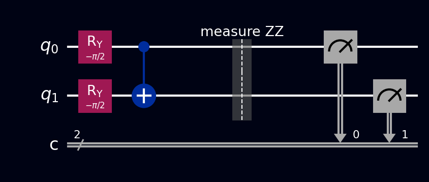
The ZZ measurement circuit at the optimal angle \( \theta = -\pi/2 \). Barriers separate the ansatz (state preparation) from the measurement. For the XX and YY circuits, add the appropriate basis rotations between the barrier and the measurement (see The circuit above).
OPENQASM 2.0;
include "qelib1.inc";

qreg q[2];
creg c[2];

// Ansatz: prepare the trial state
x q[1];
ry(-pi/2) q[0];
cx q[0], q[1];
barrier q;

// ZZ measurement (no basis rotation needed)
measure q -> c;
OPENQASM 3.0;
include "stdgates.inc";

qubit[2] q;
bit[2] c;

// Ansatz: prepare the trial state
x q[1];
ry(-pi/2) q[0];
cx q[0], q[1];
barrier q;

// ZZ measurement
c = measure q;
from qiskit import QuantumCircuit
from qiskit_aer import AerSimulator
from scipy.optimize import minimize

sim = AerSimulator()

def ansatz(theta):
    """Tunable Bell-state recipe: at theta = -pi/2 this is |Psi->."""
    qc = QuantumCircuit(2)
    qc.x(1)
    qc.ry(theta, 0)
    qc.cx(0, 1)
    return qc

def measure_term(theta, basis):
    """Measure one Pauli term. H rotates X->Z; Sdg+H rotates Y->Z."""
    qc = ansatz(theta)
    if basis == "XX":
        qc.h([0, 1])
    elif basis == "YY":
        qc.sdg([0, 1])
        qc.h([0, 1])
    qc.measure_all()
    counts = sim.run(qc, shots=2048).result().get_counts()
    # Parity trick: even number of 1s -> +1, odd -> -1
    signed = sum(shots if bits.count("1") % 2 == 0 else -shots
                 for bits, shots in counts.items())
    return signed / 2048

def energy(params):
    return sum(measure_term(params[0], b) for b in ["XX", "YY", "ZZ"])

# Expected output: theta ~ -1.57, energy ~ -3
result = minimize(energy, x0=[0.1], method="COBYLA")
print("theta =", result.x[0], " energy =", result.fun)
import cirq
import numpy as np

q = cirq.LineQubit.range(2)

circuit = cirq.Circuit()
# Ansatz: prepare the trial state
circuit.append(cirq.X(q[1]))
circuit.append(cirq.ry(-np.pi / 2).on(q[0]))
circuit.append(cirq.CNOT(q[0], q[1]))
circuit.append(cirq.ops.Moment())  # barrier

# ZZ measurement
circuit.append(cirq.measure(*q, key='result'))
print(circuit)
namespace QompileCircuit {
    open Microsoft.Quantum.Canon;
    open Microsoft.Quantum.Intrinsic;
    open Microsoft.Quantum.Math;

    operation Circuit() : Result[] {
        use q = Qubit[2];
        mutable c = [Zero, size = 2];

        // Ansatz: prepare the trial state
        X(q[1]);
        Ry(-PI() / 2.0, q[0]);
        CNOT(q[0], q[1]);

        // ZZ measurement
        set c w/= 0 <- M(q[0]);
        set c w/= 1 <- M(q[1]);

        ResetAll(q);
        return c;
    }
}
What you'll see¶
- Probabilities - at the optimum, two 50% bars on
01and10in the ZZ circuit - and the same anticorrelated pattern in the XX and YY circuits. Only the entangled singlet disagrees in every measurement basis at once; no product state can do that. - Q-Sphere - on the bare preparation circuit: two points with opposite phase colors, the literal \( |\Psi^-\rangle \) picture from the Bell states page. At \( \theta = 0 \), a single point on \( |01\rangle \) - watch entanglement appear as you tune the knob.
- Statevector - two amplitudes of magnitude ≈0.707 with opposite signs on \( |01\rangle \) and \( |10\rangle \) at the optimum; at intermediate \( \theta \), unequal magnitudes that show the optimizer partway through its journey.