QAOA
The Quantum Approximate Optimization Algorithm attacks combinatorial optimization problems - scheduling, routing, portfolio selection, network partitioning - by teaming a small, shallow quantum circuit with an ordinary classical optimizer. It's one of the flagship algorithms for today's noisy, limited-qubit hardware, because the circuit stays short and the classical computer does the heavy lifting of tuning it.
Why this exists
Combinatorial optimization problems share a painful shape: an enormous number of candidate solutions (bitstrings), a score for each one, and no better classical strategy in general than clever variations on "try lots of them." Many of these problems are NP-hard, and nobody expects any computer, quantum or classical, to solve them exactly and efficiently.
QAOA aims for something more modest and more practical: good solutions, fast. It prepares a quantum state that concentrates probability on high-scoring bitstrings, so that measuring it gives you very good candidates with high likelihood. The state is prepared by a circuit with a handful of tunable knobs, and a classical optimizer turns those knobs to make the measured scores as good as possible.
The standard showcase problem, used on this page, is MaxCut: given a network of nodes and edges, split the nodes into two groups so that as many edges as possible run between the groups.
What you need to know first
- Cost functions. Every optimization problem gets encoded as a function \( C(z) \) that scores each bitstring \( z \). For MaxCut: assign each node a bit (which group it's in), and \( C(z) \) counts the edges whose endpoints got different bits.
- Cost Hamiltonians. A Hamiltonian is an operator whose role here is simple: it's the quantum version of the score sheet. Encode the cost so that each basis state \( |z\rangle \) is scored by \( C(z) \). The useful building block is the observation that \( Z_i Z_j \) (a Pauli-Z on qubits \( i \) and \( j \)) gives \( +1 \) when bits \( i \) and \( j \) agree and \( -1 \) when they differ - a one-term "is this edge cut?" detector. (VQE discusses Hamiltonians and expectation values in more depth.)
- Expectation values. \( \langle C \rangle \) is just the average score of the bitstrings you'd get by measuring the state many times. That's the number the classical optimizer tries to push up, and it's estimated directly from measurement counts.
- A classical optimizer. Anything that minimizes a function of a few real variables - even a grid search works for the two-parameter version here.
How it works, step by step
The circuit has \( p \) layers (the "depth"); each layer has two knobs, an angle \( \gamma \) for the cost step and \( \beta \) for the mixer step. This page uses \( p = 1 \): two knobs total.
- Superpose: H on every qubit - every possible grouping of the nodes, all at once, equally weighted.
- Cost layer (knob \( \gamma \)): for each edge \( (i, j) \), apply RZZ\( (2\gamma) \) between qubits \( i \) and \( j \). This stamps each bitstring-branch with a phase proportional to its score - good cuts and bad cuts start to spin apart in phase.
- Mixer layer (knob \( \beta \)): RX\( (2\beta) \) on every qubit. Phases alone are invisible to measurement (a lesson from Grover's); the mixer converts the phase differences into amplitude differences, letting branches interfere so that high-scoring strings become more likely.
- Measure all qubits, many shots, and compute the average cut value of the results.
- Classical loop: an ordinary optimizer adjusts \( (\gamma, \beta) \) to maximize that average, re-running the circuit each try. When it converges, sample once more and keep the best bitstring seen.
Deeper circuits (\( p = 2, 3, \ldots \)) alternate more cost and mixer layers with their own knobs, approximating the ideal annealing process better at the price of a longer circuit.
The math
For MaxCut the cost function is
using the \( \pm1 \) convention for bits (node in group A = \( +1 \), group B = \( -1 \)): each edge term is 1 when the endpoints differ, 0 when they agree. Promote each \( z_i \) to the operator \( Z_i \) and this becomes the cost Hamiltonian \( C \to H_C \). The QAOA state with one layer is
where \( H_M = \sum_i X_i \) is the mixer. The exponentials sound abstract but compile to plain gates: each edge's \( e^{-i\gamma Z_i Z_j} \) is exactly one RZZ\( (2\gamma) \) gate, and each \( e^{-i\beta X_i} \) is one RX\( (2\beta) \). The classical optimizer maximizes \( \langle \gamma, \beta | H_C | \gamma, \beta \rangle \), which is estimated by averaging \( C \) over measurement outcomes - no operator algebra needed at runtime.
A worked example
Use the smallest interesting graph: a triangle - nodes 0, 1, 2, edges (0,1), (1,2), (0,2). Enumerate the eight groupings: 000 and 111 keep all nodes together (cut value 0); every other bitstring isolates one node and cuts 2 of the 3 edges (cut value 2, the maximum - you can never cut all 3 edges of a triangle, since some pair must land in the same group).
So the optimizer's job is to make the six value-2 strings likely and 000/111 rare. Run the \( p = 1 \) circuit and you'll find the average cut peaks around \( \gamma \approx 0.79, \beta \approx 0.39 \) (about \( \pi/4 \) and \( \pi/8 \)), where \( \langle C \rangle \approx 1.5 \) and the two worthless strings have visibly suppressed probability. Measuring then gives a maximum cut with high probability - and any of the six is a correct answer.
The circuit
For the triangle at fixed \( (\gamma, \beta) = (0.79, 0.39) \), build on 3 qubits (or load QAOA from the Ready algorithms panel):
- H on
q[0],q[1],q[2] - Cost layer: RZZ(1.58) on the pair (
q[0],q[1]), then (q[1],q[2]), then (q[0],q[2]) - one per edge, angle \( 2\gamma \) - Mixer layer: RX(0.78) on each of the three qubits - angle \( 2\beta \)
- Measure all three qubits
In Qompile you set the two angles by hand; the "classical loop" is you trying different values and watching the average improve, which is a genuinely good way to feel what the optimizer does.
References for the circuit layout: Wikipedia: Quantum optimization algorithms and IBM Quantum Learning: Variational algorithm design.
The circuit in code
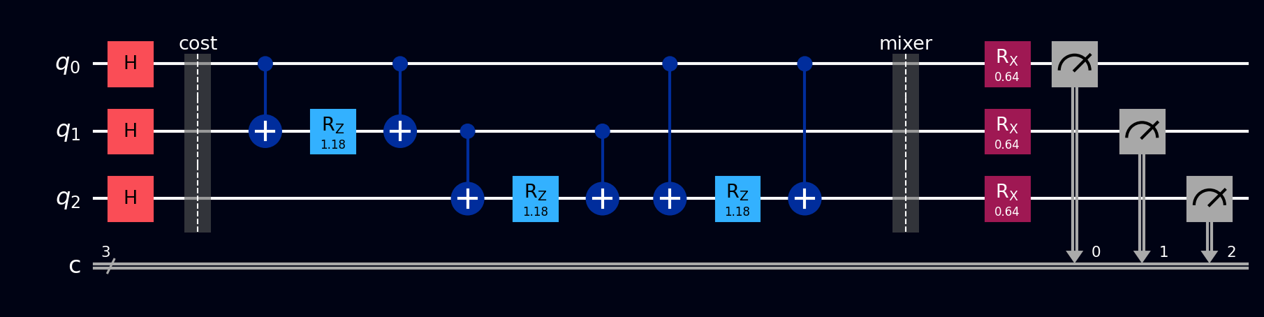
The triangle MaxCut circuit at \( (\gamma, \beta) = (0.79, 0.39) \). Barriers separate the three phases: superposition, cost layer, and mixer layer + measurement.
OPENQASM 2.0;
include "qelib1.inc";

qreg q[3];
creg c[3];

// Superpose
h q[0];
h q[1];
h q[2];
barrier q;

// Cost layer: RZZ(2*gamma) on each edge, gamma = 0.79
rzz(1.58) q[0], q[1];
rzz(1.58) q[1], q[2];
rzz(1.58) q[0], q[2];
barrier q;

// Mixer layer: RX(2*beta) on each qubit, beta = 0.39
rx(0.78) q[0];
rx(0.78) q[1];
rx(0.78) q[2];

measure q -> c;
OPENQASM 3.0;
include "stdgates.inc";

qubit[3] q;
bit[3] c;

// Superpose
h q[0];
h q[1];
h q[2];
barrier q;

// Cost layer: RZZ(2*gamma) on each edge
rzz(1.58) q[0], q[1];
rzz(1.58) q[1], q[2];
rzz(1.58) q[0], q[2];
barrier q;

// Mixer layer: RX(2*beta) on each qubit
rx(0.78) q[0];
rx(0.78) q[1];
rx(0.78) q[2];

c = measure q;
from qiskit import QuantumCircuit
from qiskit_aer import AerSimulator
from scipy.optimize import minimize

edges = [(0, 1), (1, 2), (0, 2)]  # triangle graph
n = 3
sim = AerSimulator()

def qaoa_circuit(gamma, beta):
    qc = QuantumCircuit(n, n)
    qc.h(range(n))                    # every grouping, equally weighted
    for i, j in edges:                # one RZZ per edge scores the cut
        qc.rzz(2 * gamma, i, j)
    qc.rx(2 * beta, range(n))         # mixer converts phases to amplitudes
    qc.measure(range(n), range(n))
    return qc

def cut_value(bits):
    return sum(1 for i, j in edges if bits[i] != bits[j])

def average_cut(params):
    counts = sim.run(qaoa_circuit(*params), shots=2048).result().get_counts()
    total = sum(cut_value(key[::-1]) * shots for key, shots in counts.items())
    return -total / 2048              # negative because optimizers minimize

# COBYLA is gradient-free, suits noisy objective estimates
result = minimize(average_cut, x0=[0.5, 0.5], method="COBYLA")
print("best (gamma, beta):", result.x, " average cut:", -result.fun)

# The six max-cut strings dominate; 000/111 trail far behind
counts = sim.run(qaoa_circuit(*result.x), shots=2048).result().get_counts()
print(sorted(counts.items(), key=lambda kv: -kv[1]))
import cirq

q = cirq.LineQubit.range(3)
edges = [(0, 1), (1, 2), (0, 2)]
gamma, beta = 0.79, 0.39

circuit = cirq.Circuit()
# Superpose
circuit.append([cirq.H(q[i]) for i in range(3)])
circuit.append(cirq.ops.Moment())  # barrier

# Cost layer: RZZ(2*gamma) on each edge
for i, j in edges:
    circuit.append(cirq.ZZPowGate(exponent=2 * gamma / 3.14159).on(q[i], q[j]))
circuit.append(cirq.ops.Moment())  # barrier

# Mixer layer: RX(2*beta) on each qubit
circuit.append([cirq.rx(2 * beta).on(q[i]) for i in range(3)])

circuit.append(cirq.measure(*q, key='result'))
print(circuit)
namespace QompileCircuit {
    open Microsoft.Quantum.Canon;
    open Microsoft.Quantum.Intrinsic;
    open Microsoft.Quantum.Math;

    operation Circuit() : Result[] {
        use q = Qubit[3];
        mutable c = [Zero, size = 3];

        let gamma = 0.79;
        let beta = 0.39;

        // Superpose
        H(q[0]);
        H(q[1]);
        H(q[2]);

        // Cost layer: Rzz(2*gamma) on each edge
        Exp([PauliZ, PauliZ], gamma, [q[0], q[1]]);
        Exp([PauliZ, PauliZ], gamma, [q[1], q[2]]);
        Exp([PauliZ, PauliZ], gamma, [q[0], q[2]]);

        // Mixer layer: Rx(2*beta) on each qubit
        Rx(2.0 * beta, q[0]);
        Rx(2.0 * beta, q[1]);
        Rx(2.0 * beta, q[2]);

        set c w/= 0 <- M(q[0]);
        set c w/= 1 <- M(q[1]);
        set c w/= 2 <- M(q[2]);

        ResetAll(q);
        return c;
    }
}
What you'll see
- Probabilities - at good \( (\gamma, \beta) \): six healthy bars on the cut-value-2 strings and two suppressed bars on
000and111. At \( \gamma = \beta = 0 \) the histogram is perfectly flat - the knobs really are what create the bias. - Q-Sphere - after the cost layer, all eight branches with phase colors grouped by cut value (this is the score, written in phase); the mixer then converts that pattern into the size differences you see at the end.
- Statevector - amplitudes cluster into two magnitude classes matching the two cost classes; watch them separate as you increase \( \gamma \) from zero.