QPE
Quantum Phase Estimation measures a quantity that is otherwise invisible: the phase a quantum operation imprints on its special states. That sounds niche, but it's the workhorse subroutine of the field - Shor's algorithm is QPE pointed at arithmetic, and quantum chemistry's most accurate energy methods are QPE pointed at molecules. If you learn one "advanced" algorithm deeply, make it this one.
Why this exists
Many hard problems can be rephrased as: "here's an operation \( U \) I can run; tell me the phase it applies to one of its eigenstates." The period of modular multiplication (the heart of factoring), the energy levels of a molecule, the long-run behavior of a quantum walk - all of them hide inside such phases. The catch is that a phase is not directly measurable: a state \( e^{2\pi i\varphi}|\psi\rangle \) gives exactly the same measurement statistics as \( |\psi\rangle \). Phases only become visible through interference.
QPE is the standard machine for making that happen. Given a unitary \( U \) and an eigenstate \( |\psi\rangle \) with
QPE writes the number \( \varphi \), in binary, onto a register of ordinary measurable qubits. More counting qubits = more binary digits = more precision.
What you need to know first
Unitary gates
Every quantum gate is a unitary operation - a matrix \( U \) satisfying \( U^\dagger U = I \) (its conjugate-transpose is its inverse). Two consequences matter here: unitaries are reversible (nothing is lost, you can always undo them), and they preserve lengths (probabilities still sum to 1 afterward). Think of them as rotations of the state space - nothing gets stretched, squashed, or erased. Background on matrices and their inverses: Khan Academy's matrices unit.
Eigenvectors and eigenvalues
An eigenvector of an operation is a state the operation doesn't move - it only gets scaled by a number, the eigenvalue:
Khan Academy's introduction to eigenvalues and eigenvectors builds the general idea. For unitary operations there's a twist that makes QPE possible: because lengths are preserved, the eigenvalue can't grow or shrink anything, so it must have absolute value 1 - it can only be a rotation in phase, \( \lambda = e^{2\pi i\varphi} \). Every unitary eigenvalue is a point on the unit circle, pinned down by the single real number \( \varphi \). (Complex numbers refresher if needed.)
A concrete example, used throughout this page: the T gate leaves \( |0\rangle \) alone and maps \( |1\rangle \mapsto e^{i\pi/4}|1\rangle \). So \( |1\rangle \) is an eigenstate of T with \( e^{2\pi i \varphi} = e^{i\pi/4} \), i.e. \( \varphi = \frac{1}{8} \).
Binary fractions
QPE returns \( \varphi \) as a binary fraction: with 3 counting qubits reading \( b_1 b_2 b_3 \), the estimate is \( \varphi \approx \frac{b_1}{2} + \frac{b_2}{4} + \frac{b_3}{8} \). Our target \( \varphi = \frac{1}{8} \) is \( 0.001 \) in binary - exactly representable in 3 bits, so the answer will come out exact.
Controlled operations and phase kickback
QPE runs \( U \) as a controlled operation (control modifier: apply \( U \) only if a control qubit is \( |1\rangle \)). When the target sits in an eigenstate, controlled-\( U \) can't change it - but the eigenvalue phase sneaks backward onto the control qubit: \( |1\rangle_c|\psi\rangle \mapsto e^{2\pi i\varphi}|1\rangle_c|\psi\rangle \), while \( |0\rangle_c|\psi\rangle \) is untouched. A control in superposition therefore becomes \( \frac{|0\rangle + e^{2\pi i\varphi}|1\rangle}{\sqrt{2}} \): the phase now lives on a qubit we control and can interfere. This is the same phase kickback introduced in Deutsch-Jozsa, in its general form.
How it works, step by step
Registers: \( t \) counting qubits (precision) plus enough qubits to hold the eigenstate \( |\psi\rangle \).
- Prepare the eigenstate on the target register.
- Superpose the counters: H on every counting qubit.
- Controlled powers of \( U \): counting qubit \( j \) controls \( U^{2^j} \) - the first controls \( U \), the second \( U^2 \), the third \( U^4 \), and so on. By phase kickback, counting qubit \( j \) picks up phase \( e^{2\pi i (2^j \varphi)} \). Collectively, the counting register now holds the number \( \varphi \) encoded in phases - one binary-digit's worth of rotation per qubit.
- Inverse QFT on the counting register. The Quantum Fourier Transform is the unitary that converts between "number stored in phases" and "number stored as a plain bitstring"; its inverse decodes our phase pattern into a readable binary number. (It's the same H-converts-phases-to-bits idea from Bernstein-Vazirani, upgraded with the twisty P rotations needed for multi-digit binary place value.)
- Measure the counting register: read integer \( m \), estimate \( \varphi \approx \frac{m}{2^t} \).
If \( \varphi \) fits exactly in \( t \) binary digits, the result is exact and deterministic. If not, the measurement concentrates on the nearest \( t \)-bit value (better than 40% for the single nearest, and overwhelmingly likely to be within one step of it) - run a few shots and take the consensus.
A worked example
Estimate the T gate's phase on eigenstate \( |1\rangle \), with \( t = 3 \) counting qubits. Target answer: \( \varphi = \frac{1}{8} \), binary \( 0.001 \).
After step 2, each counting qubit is \( \frac{|0\rangle + |1\rangle}{\sqrt{2}} \). Step 3 kicks phases back:
- qubit 0 (controls \( T^1 \)): \( \frac{|0\rangle + e^{2\pi i/8}|1\rangle}{\sqrt 2} \)
- qubit 1 (controls \( T^2 \)): \( \frac{|0\rangle + e^{2\pi i/4}|1\rangle}{\sqrt 2} \)
- qubit 2 (controls \( T^4 \)): \( \frac{|0\rangle + e^{2\pi i/2}|1\rangle}{\sqrt 2} \)
Each qubit holds one binary digit of \( \varphi \), encoded as "how far around the circle" its phase has turned. The inverse QFT decodes the pattern, and the register reads \( 001 \) - the integer 1 - giving \( \varphi = \frac{1}{8} \) exactly, on every shot. Swap the T for an S gate (\( \varphi = \frac{1}{4} \)) and the readout becomes \( 010 \); the machine really is printing the phase in binary.
The circuit
Build on 4 qubits: q[0]-q[2] counting, q[3] the eigenstate. Controlled-T powers are P gates with a control attached (T = P(\( \pi/4 \)), so T² = P(\( \pi/2 \)) and T⁴ = P(\( \pi \))). Or load QPE from the Ready algorithms panel.
- Eigenstate: X on
q[3] - Superpose: H on
q[0],q[1],q[2] - Controlled powers: controlled-P(\( \pi/4 \)) from
q[0]toq[3]; controlled-P(\( \pi/2 \)) fromq[1]toq[3]; controlled-P(\( \pi \)) fromq[2]toq[3] - Inverse QFT on
q[0]-q[2], gate by gate: SWAPq[0]↔q[2]; Hq[0]; controlled-P(\( -\pi/2 \))q[0]→q[1]; Hq[1]; controlled-P(\( -\pi/4 \))q[0]→q[2]; controlled-P(\( -\pi/2 \))q[1]→q[2]; Hq[2] - Measure
q[0]-q[2]- reads001, i.e. \( \varphi = 1/8 \)
References for the circuit layout: Wikipedia: Quantum phase estimation algorithm and IBM Quantum Learning: Phase estimation and factoring.
The circuit in code
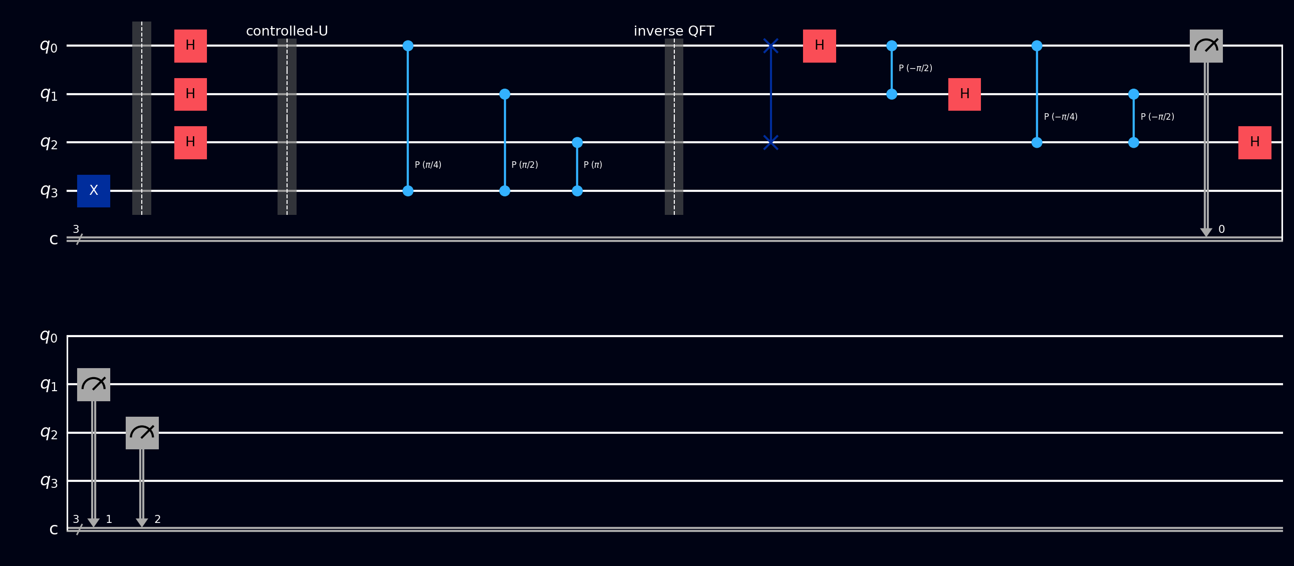
The T-gate QPE circuit (\( t = 3 \) counting qubits, 1 target, \( \varphi = 1/8 \)). Barriers separate the three phases: eigenstate + superposition, controlled phase kicks, and inverse QFT + measurement.
OPENQASM 2.0;
include "qelib1.inc";

qreg q[4];
creg c[3];

// Eigenstate |1> on the target
x q[3];

// Superpose counting register
h q[0];
h q[1];
h q[2];
barrier q;

// Controlled powers of T = P(pi/4)
cp(pi/4) q[0], q[3];    // T^1
cp(pi/2) q[1], q[3];    // T^2
cp(pi) q[2], q[3];      // T^4
barrier q;

// Inverse QFT on counting register
swap q[0], q[2];
h q[0];
cp(-pi/2) q[0], q[1];
h q[1];
cp(-pi/4) q[0], q[2];
cp(-pi/2) q[1], q[2];
h q[2];

measure q[0] -> c[0];
measure q[1] -> c[1];
measure q[2] -> c[2];
OPENQASM 3.0;
include "stdgates.inc";

qubit[4] q;
bit[3] c;

// Eigenstate |1> on the target
x q[3];

// Superpose counting register
h q[0];
h q[1];
h q[2];
barrier q;

// Controlled powers of T = P(pi/4)
cp(pi/4) q[0], q[3];
cp(pi/2) q[1], q[3];
cp(pi) q[2], q[3];
barrier q;

// Inverse QFT on counting register
swap q[0], q[2];
h q[0];
cp(-pi/2) q[0], q[1];
h q[1];
cp(-pi/4) q[0], q[2];
cp(-pi/2) q[1], q[2];
h q[2];

c[0] = measure q[0];
c[1] = measure q[1];
c[2] = measure q[2];
from math import pi
from qiskit import QuantumCircuit
from qiskit.circuit.library import QFT
from qiskit_aer import AerSimulator

t = 3                                  # counting qubits (= binary digits of precision)
qc = QuantumCircuit(t + 1, t)

# QPE needs the eigenstate handed to it — here that's trivial (|1>)
qc.x(t)

# Superpose the counting register
qc.h(range(t))
qc.barrier()

# Powers-of-two ladder: counting qubit j controls U^(2^j).
# For T = P(pi/4), running it 2^j times = one P gate with 2^j× the angle.
for j in range(t):
    qc.cp(pi / 4 * 2**j, j, t)
qc.barrier()

# The decoder: inverse QFT converts "number stored in phases"
# into a readable binary number (includes qubit-reversal swaps)
qc.append(QFT(t, inverse=True), range(t))

qc.measure(range(t), range(t))

# Readout: integer m, then phi = m / 2^t
counts = AerSimulator().run(qc, shots=1024).result().get_counts()
m = int(max(counts, key=counts.get), 2)
print(counts)          # {'001': 1024}
print("phase =", m / 2**t)  # 0.125 — exact because 1/8 fits in 3 bits
import cirq
import numpy as np

q = cirq.LineQubit.range(4)

circuit = cirq.Circuit()
# Eigenstate |1> on the target
circuit.append(cirq.X(q[3]))

# Superpose counting register
circuit.append([cirq.H(q[i]) for i in range(3)])
circuit.append(cirq.ops.Moment())  # barrier

# Controlled powers of T = P(pi/4)
for j in range(3):
    angle = np.pi / 4 * 2**j
    circuit.append(cirq.CZPowGate(exponent=angle / np.pi).on(q[j], q[3]))
circuit.append(cirq.ops.Moment())  # barrier

# Inverse QFT on counting register (hand-built for 3 qubits)
circuit.append(cirq.SWAP(q[0], q[2]))
circuit.append(cirq.H(q[0]))
circuit.append(cirq.CZPowGate(exponent=-0.5).on(q[0], q[1]))
circuit.append(cirq.H(q[1]))
circuit.append(cirq.CZPowGate(exponent=-0.25).on(q[0], q[2]))
circuit.append(cirq.CZPowGate(exponent=-0.5).on(q[1], q[2]))
circuit.append(cirq.H(q[2]))

circuit.append(cirq.measure(q[0], q[1], q[2], key='result'))
print(circuit)
namespace QompileCircuit {
    open Microsoft.Quantum.Canon;
    open Microsoft.Quantum.Intrinsic;
    open Microsoft.Quantum.Math;

    operation Circuit() : Result[] {
        use q = Qubit[4];
        mutable c = [Zero, size = 3];

        // Eigenstate |1> on the target
        X(q[3]);

        // Superpose counting register
        H(q[0]);
        H(q[1]);
        H(q[2]);

        // Controlled powers of T = P(pi/4)
        Controlled R1([q[0]], (PI() / 4.0, q[3]));
        Controlled R1([q[1]], (PI() / 2.0, q[3]));
        Controlled R1([q[2]], (PI(), q[3]));

        // Inverse QFT on counting register
        SWAP(q[0], q[2]);
        H(q[0]);
        Controlled R1([q[0]], (-PI() / 2.0, q[1]));
        H(q[1]);
        Controlled R1([q[0]], (-PI() / 4.0, q[2]));
        Controlled R1([q[1]], (-PI() / 2.0, q[2]));
        H(q[2]);

        set c w/= 0 <- M(q[0]);
        set c w/= 1 <- M(q[1]);
        set c w/= 2 <- M(q[2]);

        ResetAll(q);
        return c;
    }
}
What you'll see
- Probabilities - one bar at 100% on
001for the exact case; a tight cluster around the true phase in the inexact case. - Phase disks - snapshot after step 3: each counting qubit sits at 50/50 but with a different phase angle on its disk - the binary digits of \( \varphi \), literally drawn as clock hands, and the clearest picture of "the answer is stored in phases" anywhere in this section.
- Statevector - after step 3, sixteen amplitudes of equal magnitude whose phases wind at different rates; after the inverse QFT, everything gathered onto a single basis state.